

baona
A few weeks ago, while backtesting an idea for a refined technical tool on the S&P 500 ETF (SPY), I discovered an error I had made in my Excel sheet. This error, however, seemed to reveal an anomaly in daily price behavior. Upon further investigation, this apparent anomaly seemed to reveal additional anomalies, all related to price behavior over the course of the average week. Some of these anomalies are already known or, more precisely, I think, partially described phenomena such as “the Weekend Effect“, ” Turnaround Tuesday“, and the “Friday Effect” – but have not been combined into a systematic whole. In this article, I am going to attempt a first approximation of a systematic description of returns distributed by portions of the week. I think the findings are original and are likely to be of interest to academics, traders, and anyone else interested in market behavior.
This article will be divided into five sections spread out over three installments:
Part 1
1. Basic claims
2. Fama-French data, 1926-2023
3. Possible implications
Part 2
4. Dow Jones data, 1885-2023
Part 3
5. Mechanics
Before delving into the argument, I should caveat this entire article by acknowledging that I have very poor statistical and math skills, I have no prior experience working with daily data, and I had no previous awareness of basic calendar anomalies such as the Weekend Effect. Therefore, there is a heightened possibility that what follows is going to be obvious, wrong, already known, or, somehow, all three.
I have tried to resolve the statistics problem by limiting my claims and trying to use rudimentary statistical tools primarily to describe the phenomena I think I have found. That is, I am not trying to “prove” anything as much as I am trying to illustrate. As for the issues relating to lack of experience or awareness of calendar effects, I have done my best to verify that the claims are original. Hopefully, readers will kindly point out where my claims/techniques are unoriginal or wrong.
A positive side effect of these issues, assuming that the observations are not misguided, is that it should make my arguments more accessible to general readers who are as mathematically inept as I am, and even if I have unintentionally exaggerated the originality of the claims, they might serve as a jumping off point for those who, like me, are unfamiliar with these phenomena.
Section 1. Basic claims
I calculated end-of-week (EOW) prices, middle-of-week (MOW) prices, and beginning-of-week (BOW) prices for twenty long-term stock return series, and I calculated the returns between each of those periods. Thus, each week for each of the series was divided into three parts (EOW/MOW, MOW/BOW, and BOW/EOW). The last one is effectively the same as that measured in the Weekend Effect.
For simplicity’s sake, one could think of EOW as being ‘Friday’, MOW as being ‘Wednesday’, and BOW as being ‘Monday’, except that markets are not always open on each of those days, and up until the 1950s, markets were often open on Saturdays. So, although I think it is perfectly acceptable to refer to this as ‘Friday’, ‘Wednesday’, and ‘Monday’, it has to be remembered that this is not precisely true.
One problem with this is identifying the ‘Wednesday’ price (the MOW price) when markets were closed on a given Wednesday. In those instances, I calculated the MOW as the average of the Tuesday and Thursday prices.
In short, I am comparing stock returns over the course of a week divided between beginning, middle, and end rather than the actual day of the week, which, as far as I am aware, is the standard approach. And, this is what I found:
- EOW/MOW > MOW/BOW > BOW/EOW: Over the long haul, returns at the end of the week have been higher than returns in the middle of the week, and those have both been higher than returns over the beginning of the week (i.e., the weekend).
- EOW/MOW and BOW/EOW are inversely correlated, even after controlling for the higher returns in the former. That is, if you detrend hypothetical end-of-week portfolios and beginning-of-week portfolios (all of the portfolios in this article are hypothetical), they are strongly and consistently inversely correlated.
- MOW/BOW tends to grow exponentially. That is, hypothetical middle-of-the-week portfolios tend to grow at a constant rate.
- The weekly betas of each of these portfolios – EOW/MOW, MOW/BOW, BOW/EOW – have surprisingly constant values across time and stock series. A mnemonic is 0.44 for the end of the week, 0.33 for the middle of the week, and 0.22 for the beginning of the week (weekend returns), respectively, or 4-3-2.
These claims appear to hold true for the six value-weighted Fama-French 2×3 portfolios formed on size and book-to-market, for one equal-weighted counterpart of those six (I did not test the others), and the value-weighted Fama-French 12 industry portfolios – each for the period July 1, 1926 to June 30, 2023 – and for the Dow Jones Industrial Average (DIA) from February 15, 1885 to June 30, 2023.
In Section 2, I will demonstrate these phenomena primarily using the 2×3 size and book-to-market portfolios to keep things from getting too unwieldy.
Before moving on to Section 2, however, I wanted to illustrate the basic problem as it appeared to me early on in my research to give a flavor of the sort of thing going on here. The following is a chart of a ticker for a bank called Silicon Valley Bank (OTCPK:SIVBQ), which went bankrupt in March.
Chart A. Silicon Valley Bank hypothetical performance when sliced into portfolios sorted by portion of the week. (Author calculations, Stockcharts.com)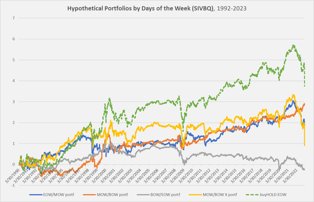
The green line represents the log stock price (indexed to 0 at the beginning of available data on Stockcharts.com) – what one would hypothetically have made by ‘buying and holding’ up until March 10 of this year. You can see the decline that began in January and then accelerated into complete collapse. The blue line (the end-of-week portfolio), partly obscured, declines in sympathy, and the grey line (the beginning-of-week portfolio) does too, but less violently. The orange line (the middle-of-week portfolio), however, keeps rising to the bitter end. The yellow line is what you get by subtracting the orange line (MOW/BOW) from the green line (the ‘buy-and-hold’ portfolio), or what you get from adding the blue and grey lines (the end-of-week and beginning-of-week portfolios).
What I intend to argue is that the orange line, the MOW/BOW portfolio, tends to rise at a near-constant rate, no matter what, across nearly all long-term historical series. This is where I began my investigation, which I then combined with the more familiar “Weekend Effect” (BOW/EOW). This then formed the basis for looking at the end-of-week (EOW/MOW) portfolio and comparing it to the other two.
Section 2. Fama-French, 1926-2023
Point 1. EOW/MOW > MOW/BOW > BOW/EOW: Returns at the end of the week, on average, have been higher than those in the middle of the week, which have been higher than those at the beginning of the week.
The following chart shows this for the Large-cap/Medium-Book-to-Market (ME2BM2) portfolio.
Chart B. The later in the week, the higher the returns historically. (Own calculations, Kenneth French data)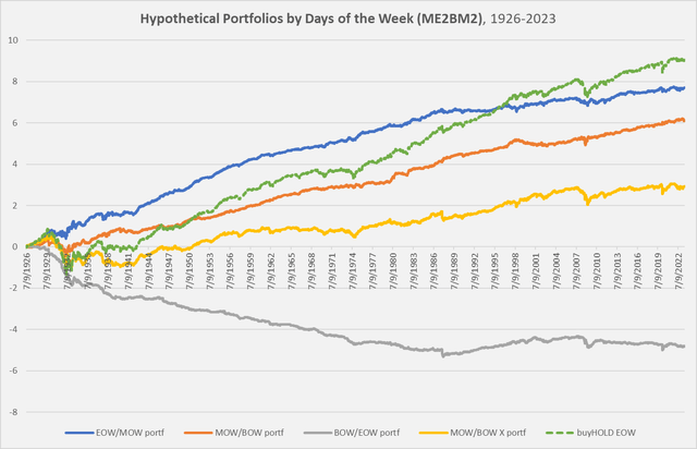
For much of the time, end-of-week returns (in blue) outperformed the entire portfolio. The following table illustrates this for each of the six portfolios across each portion of the week. EOW/MOW is almost always higher than MOW/BOW (except for Big LoBM, large-cap/low-book-to-market returns), and they all clearly exceed BOW/EOW.
Chart C. The later in the week, the higher the returns, especially in smallcaps. (Author calculations, Kenneth French data)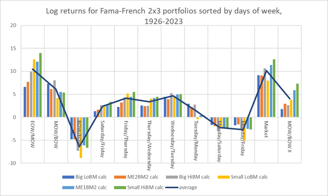
One can also see that EOW/MOW returns for small caps (yellow, light blue, and green) have historically outperformed their underlying portfolios.
Point 2. EOW/MOW and BOW/EOW are inversely correlated, even after controlling for the higher returns in the former. That is, if you detrend hypothetical end-of-week portfolios and beginning-of-week portfolios with a simple linear regression, they are strongly and consistently inversely correlated.
This time, let’s use the Small-cap/Medium-Book-to-Value (ME1BM2) portfolio.
Chart D. Late-week returns and early-week returns are inversely correlated historically. (Author calculations, Kenneth French data)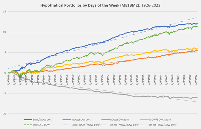
This chart is similar to the ME2BM2 one we looked at a moment ago, but it also includes trend lines for portfolios arranged by days of the week. The blue line (end-of-week returns) breaks above and below its trendline at roughly the same time that the grey line (beginning-of-week returns) breaks below and above its trendline. If we subtract each of those lines from their trendlines (leaving us with “residuals”), we get the following chart.
Chart E. Late-week and early-week portfolios have been inversely correlated when detrended (Author calculations, Kenneth French data)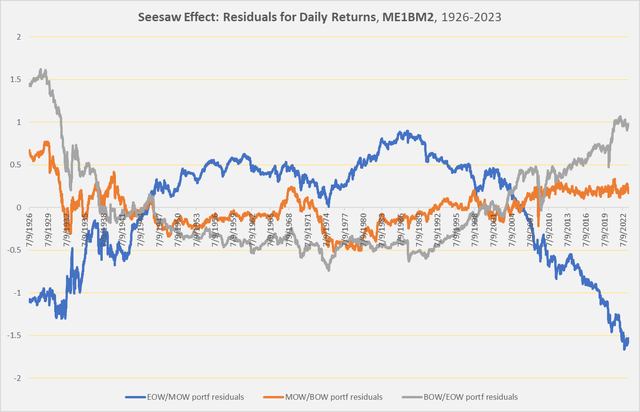
There is a clear tendency, over the long term, for end-of-week and beginning-of-the-week returns to move inversely relative to one another, on top of the secular tendency for the former to be much higher than the latter. This holds true across all portfolios.
Chart F. Correlations between detrended late-week and early-week returns are inversely correlated across 2×3 size and value Fama-French portfolios (Author calculations, Kenneth French data)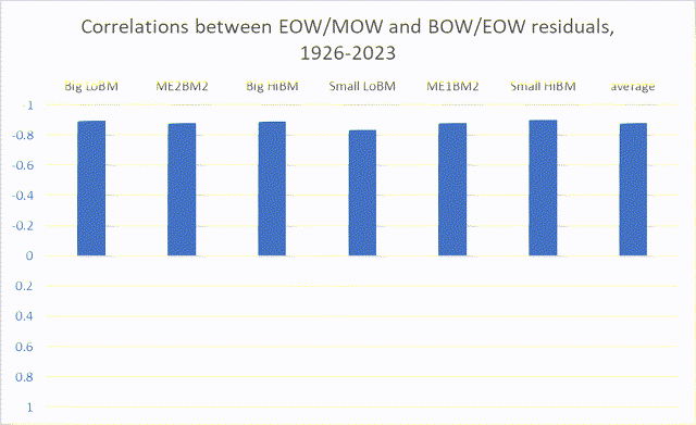
Now, let’s go back to the midweek effect we briefly looked at with Silicon Valley Bank.
Point 3. MOW/BOW tends to grow exponentially. That is, hypothetical middle-of-the-week portfolios tend to grow at a constant rate.
This may already be observable in the charts under Point 2. Notice how close the orange line (middle-of-week returns) cleaves to its trendline in Chart D. In Chart E, we can see how consistently the orange line stays at 0.
Let’s look at this with the Small-cap/High-Book-to-Market (Small HiBM) portfolios.
Chart G. Midweek returns have tended to grow exponentially. (Author calculations, Kenneth French data)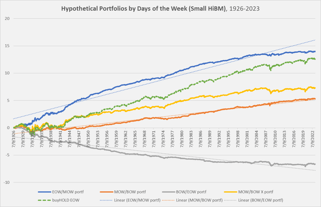
These are effectively the same patterns we saw earlier. Below is the chart of the residuals, showing the inverse correlation between end-of-week returns and beginning-of-week returns and the stability of middle-of-week returns.
Chart H. Midweek returns have smaller residuals than late-week and early-week returns. (Author calculations, Kenneth French data)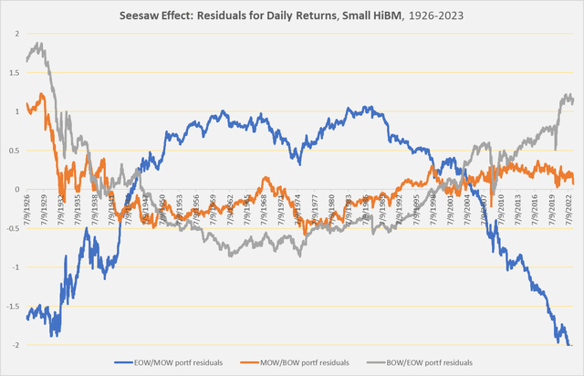
I think this is tentatively corroborated by the standard deviations of the residuals, as illustrated in the following chart. The values in the orange bars (representing the standard deviations for residuals of middle-of-week returns, MOW/BOW) are smaller than the others, most significantly the standard deviations for the end-of-week and beginning-of-week portfolios.
Chart I. Midweek returns have been much less volatile than early-week and late-week returns. (Author calculations, Kenneth French data)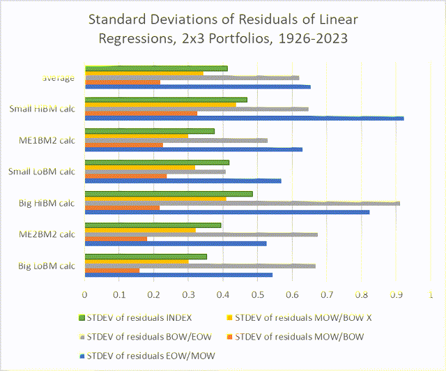
The smaller the value, the closer it sticks to its trendline. The yellow line, which measures standard deviations for portfolios of market returns less the middle-of-week returns (or, the addition of beginning-of-week and end-of-week returns) is second smallest, which might be expected if they were inversely correlated (as we found in Point 2).
So, thus far, we can say that, generally, middle-of-week (MOW/BOW) returns tend to be constant, end-of-week (EOW/MOW) returns tend to move inversely of beginning-of-week (BOW/EOW) returns, and end-of-week returns have historically tended to be fairly high (implying that beginning-of-week returns tend to be fairly low).
Let’s go on to Point 4.
Point 4. The weekly beta coefficients of each of these portfolios – EOW/MOW, MOW/BOW, BOW/EOW – have surprisingly constant values across time and stock series. A rule of thumb is 0.44 for the end of the week, 0.33 for the middle of the week, and 0.22 for the beginning of the week (weekend returns), respectively.
Actually, this rule of thumb is not quite right. If we take the betas for each of these days-of-the-week portfolios for each of the Fama-French 2×3 portfolios and calculate their averages, the actual numbers are more like 0.42 for the end of the week, 0.36 for the middle of the week, and 0.22 for the beginning of the week.
The following chart shows the betas for each of these portfolios.
Chart J. Weekly betas for the respective portfolios tend to be constant. (Author calculations, Kenneth French data)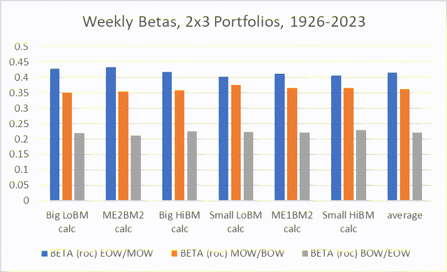
I was a little surprised at how high the betas for the MOW/BOW and BOW/EOW portfolios were. I was surprised because if the MOW/BOW portfolio rises at a constant rate, even as the market is falling, I thought this would drive it to a very low value. Similarly, with the Weekend Effect driving the BOW/EOW returns so low, I thought it would be negative.
I think I have an explanation for this, but I will save it for Section 5 on Mechanics.
To return to the topic at hand, the betas seem to hold true across time, as well. I used the 12-industry Fama-French data primarily to corroborate what I found in 2×3 data and also to look at how these factors changed over time. The following table shows betas for every full decade between 1926 and 2023 in the Business Equipment index (roughly equivalent to the Information Tech sector (XLK)).
Chart K. Betas tend to be stable over time. (Author calculations, Kenneth French data)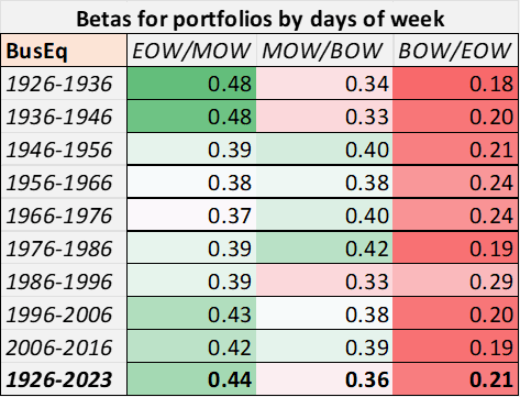
As I have argued elsewhere, the tech and energy sectors have historically been antithetical to one another. But, on this level, they seem to be in agreement.
Chart L. Betas are relatively constant across time and class. (Author calculations, Kenneth French data)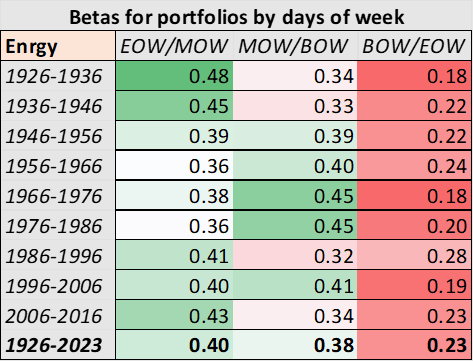
The proportions are relatively constant across indexes and time periods.
Now, let’s see what happens when we piece these four points together.
Section 3. Further Implications
1. Beta-adjusted returns
If end-of-week returns (EOW/MOW) have tended to be relatively high and its beta has tended to be somewhat lower than expected (as just discussed in Point 4 of Section 2), then its beta-adjusted returns ought to be high. Similarly, if MOW/BOW grows at a relatively constant rate, and its beta tends to remain constant over time, it should also have relatively constant beta-adjusted returns. And, if BOW/EOW has tended to be very low but has an unexpectedly high beta, its adjusted returns should be very low.
And, that does seem to be the case.
Here, I calculated adjusted returns for the Durables industry index. Adjusted returns appear to be high but volatile in EOW/MOW and low but very volatile in BOW/EOW, and high and stable in MOW/BOW.
Chart M. Beta-adjusted returns are higher later in the week and more stable in the middle of the week. (Author calculations, Kenneth French data)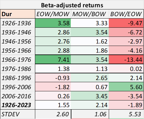
I calculated beta-adjusted returns by taking total log returns for the day-of-the-week portfolios, dividing each of them by the total log returns of the underlying index, and then dividing the respective quotients by the respective betas.
In the following chart, I show adjusted returns for the day-of-the-week portfolios in the 2×3 Fama-French series.
Chart N. Beta-adjusted intraweek returns tend to be more ‘distorted’ in small-cap stocks. (Author calculations, Kenneth French data)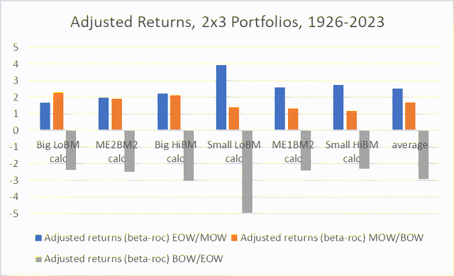
Among small-caps, adjusted returns tend to be much higher in the EOW/MOW portfolios than the MOW/BOW portfolios, whereas in the large-caps, adjusted returns are roughly equal. Large-cap growth (Big LoBM) seems to be somewhat anomalous insofar as middle-of-the-week returns appear to be significantly higher when adjusted for beta.
2. Traditional Day Effects
I think these findings suggest that there is a lot of truth behind the notions of the “Weekend Effect”, “Turnaround Tuesday”, and the “Friday Effect”, but it also suggests that these are actually epiphenomena of something larger, something at least partly captured by the four ‘rules’ described in Section 2.
Observations on the disappearance of the “Weekend Effect” are also generally accurate, unless we redefine the Weekend Effect as part of an intraweek ecosystem.
3. The MOW/BOW X portfolio
In many of the charts above, we looked at the MOW/BOW X portfolio. This is calculated by subtracting middle-of-week returns from index returns, which is the same as adding beginning-of-week and end-of-week returns. Stock prices, unfortunately, do not grow at near-constant rates while MOW/BOW portfolios do. MOW/BOW portfolios also tend to be lower than the underlying index’s returns, which means that the difference between end-of-week returns and beginning-of-week returns tends to be a small, but volatile premium above the middle-of-week returns.
The following table suggests that much of the variation in overall returns in the 2×3 portfolios can be ‘explained’ by the volatility in end-of-week returns.
Chart O. Across classes, there is greater divergence in returns in late-week portfolios. (Author calculations, Kenneth French data)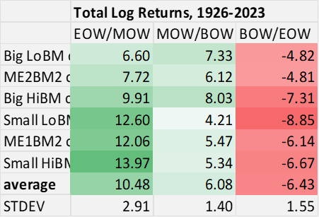
In short, these three portfolios sort of represent the three faces of the stock market. High, volatile gains (EOW/MOW); relentless, stocks-for-the-long-run ascent (MOW/BOW); and occasional shocks (BOW/EOW).
4. Trading implications
I have found at least one example of a trading strategy (at QuantifiedStrategies.com) that seems to try to capitalize on the steady accretions of the mid-week behavior and combine it with the higher volatility later in the week. As best I understand it, the strategy involves buying on a Monday or Tuesday low close and then selling on a subsequent high close. I made some small tweaks to the rules and backtested it on the SPY from 1993-2023, and it was able to beat the ETF, if it were assumed that all trades were frictionless.
Chart P. At least one trading strategy appears to be partly based on the midweek effect. (Own calculations, Stockcharts.com)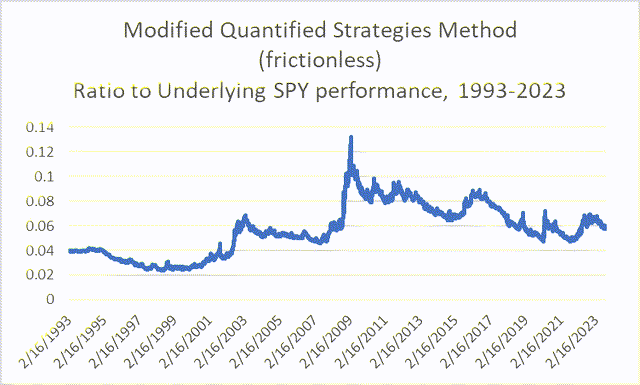
And, if adjusted for beta, the strategy appeared to beat SPY up until the friction was around 0.3% per trade, as suggested by its countercyclical behavior in the chart below.
Chart Q. Very low beta can offset underperformance and high-frequency trading to a certain extent. (Author calculations, Stockcharts.com)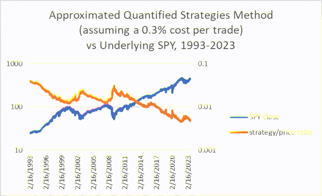
It appears to vastly outperform a strategy of Buy-Monday/Sell-Wednesday (i.e., MOW/BOW), both because of the effectiveness of the strategy and the (relatively) low frequency of trading.
Chart R. Lower frequency, stricter trading system’s hypothetical returns beat BOW/EOW strategy. (Author calculations, Stockcharts.com)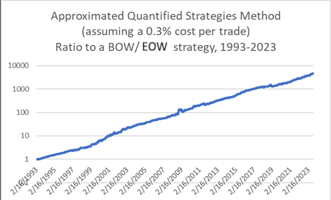
I am not advocating any trading strategy here whatsoever, but there may be ways to take some of the underlying dynamics outlined in this article and use them to develop high-frequency trading strategies, make marginal improvements to other strategies, or build low-beta products (somewhat akin to the Nightshares ETFs which attempt to lower downside risk via the ” Night Effect”).
5. Random Walks
The existence of the traditional Weekend Effect and similar such “calendar anomalies” has been used as an argument against the Efficient Market Hypothesis (or, EMH) and the random walk hypothesis, which says that any given price movement should be independent of prior price movements. If the observations in this article are correct, they would at least challenge the core premise of the EMH by suggesting an ecosystem of interrelated price movements, thereby undermining the idea that changes in stock prices are unrelated to one another. However, the patterns described thus far would have to be subjected to more rigorous statistical tests to determine the probability of them being mathematical quirks. In the Mechanics section, I am going to try to make my case for why I suspect that that is the case, but I do not have the mathematical wherewithal to prove that beyond a reasonable doubt.
Summary
In this first installment, I have tried to illustrate the basic patterns that govern returns over the course of an average week. To summarize:
- The later in the week, the higher the returns tend to be.
- End-of-week returns tend to be inversely correlated with beginning-of-week returns over the long run, even when we adjust for the behavior just described in Point 1.
- Middle-of-week returns tend to rise at a constant rate over the long term.
- The betas for hypothetical portfolios formed around times of the week roughly approximate ratio of 4:3:2 as we descend from the end of the week to the beginning of the week, and this ratio is relatively constant across portfolios and time.
This was done primarily using charts and data drawn from an examination of 19 Fama-French daily series.
Subsequently, I tried to draw out some implications of these patterns with respect to whether or not they are exploitable, whether it be by looking at adjusted returns, trading strategies, or implications for trading theory.
In Parts 2 and 3, sections 4 and 5, I will mirror this pattern insofar as I try, first, to extend these patterns to a longer data set, the Dow Jones Industrial Average from 1885 to 2023, and, second, attempt to what will necessarily be, at best, a partial description of the mechanics.
Editor’s Note: This article discusses one or more securities that do not trade on a major U.S. exchange. Please be aware of the risks associated with these stocks.


")


